A look at Biontech/Pfizer's Bayesian analysis of their Covid-19 vaccine trial

Let’s take again a look at Biontech / Pfizers vaccine candiate for which a press release stated more than 90% efficacy. As noted in my previous post Biontech/Pfizer actually use a Bayesian approach to assess the efficacy of their vaccine candiate.

In their study plan we find the following relatively short descriptions:

“The criteria for success at an interim analysis are based on the posterior probability (ie, P[VE > 30% given data]) at the current number of cases. Overwhelming efficacy will be declared if the posterior probability is higher than the success threshold. The success threshold for each interim analysis will be calibrated to protect overall type I error at 2.5%.”

“Bayesian approaches require specification of a prior distribution for the possible values of the unknown vaccine effect, thereby accounting for uncertainty in its value. A minimally informative beta prior, beta(0.700102, 1), is proposed for θ = (1-VE)/(2-VE). The prior is centered at θ = 0.4118 (VE=30%) which can be considered pessimistic. The prior allows considerable uncertainty; the 95% interval for θ is (0.005, 0.964) and the corresponding 95% interval for VE is (-26.2, 0.995).”

The approach is described in more detail in a statistical analysis plan. I could not find that plan in the internet, however. But let’s try to make an educated guess about their analysis from the information above.

Let $\pi_v$ and $\pi_c$ be the population probabilities that a vaccinated subject or a subject in the control group, respectively, fall ill to Covid-19. Then the population vaccine efficacy is given by

In their study plan Biontech/Pfizer assume a prior distribution for a parameter

Plugging in the definition of the population vaccine efficacy VE, we can rewrite $\theta$ as

Given that Biontech/Pfizer assigned the same number of subjects to the treatment and control group, this $\theta$ should denote the probability that a subject who fell ill with Covid-19 is from the treatment group, while $1-\theta$ is the probability that the subject is from the control group.

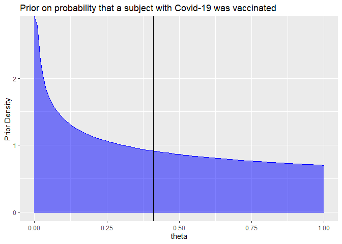
As we can see from the study plan, the assumed prior distribution of $\theta$ is a Beta distribution with shape parameters $a=a_0=0.700102$ and $b=b_0=1$. We see from the description of the beta distribution that the prior mean of $\theta$ is thus given by

Given that we have

The efficacy at the expected prior value of $\theta=0.4118$ is indeed 30% as stated by Biontech/Pfizer.

The following plot shows the prior distribution for $\theta$

a0 = 0.700102; b0 = 1
ggplot(data = data.frame(x = c(0, 1)), aes(x)) +
  stat_function(geom="area",fun = dbeta, n = 101,
    args = list(shape1 = a0, shape2 = b0),
    col="blue", fill="blue", alpha=0.5
  ) +
  ylab("Prior Density") + xlab("theta") + geom_vline(xintercept=0.4118)+
  ggtitle("Prior on probability that a subject with Covid-19 was vaccinated")

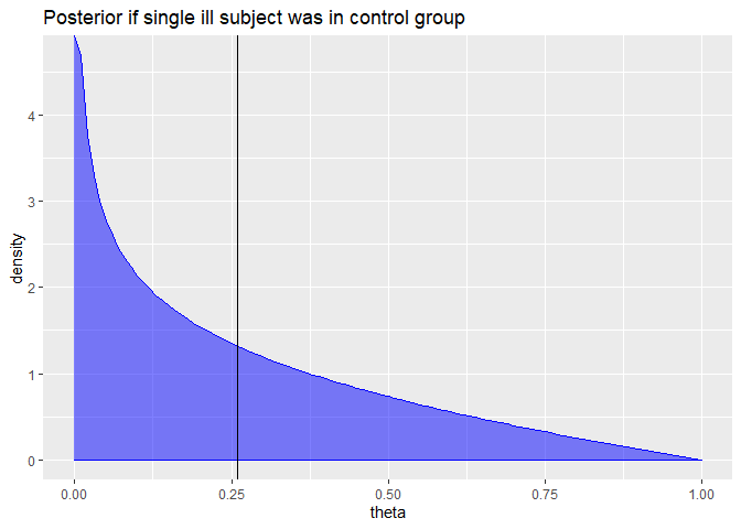
Now the crucial part of Bayesian statistics is how we update our believed distribution of $\theta$ once we get new data. Assume $m$ subjects fell ill with Covid-19 of which $m_v$ were vaccinated and $m_c$ were in the control group. Then one can show (see e.g. here) that the posterior distribution of $\theta$ is again a Beta distribution with arguments $a=a_0+m_v$ and $b=b_0+m_c$. Nice and simple!

For example, here is the posterior if we had a single observation of an ill subject and that subject was in the control group:

a = a0; b = b0+1
ggplot(data = data.frame(x = c(0, 1)), aes(x)) +
  stat_function(geom="area",fun = dbeta, n = 101,
    args = list(shape1 = a, shape2 = b),
    col="blue", fill="blue", alpha=0.5
  ) +
  xlab("theta") + ylab("density") + geom_vline(xintercept=a/(a+b)) +
  ggtitle("Posterior if single ill subject was in control group")

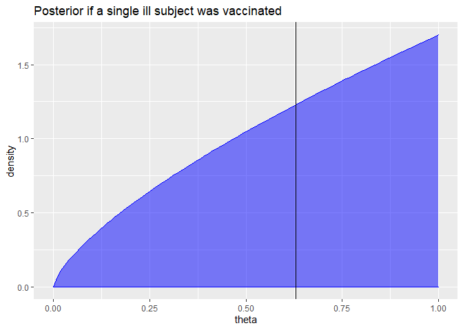
Here is the posterior if the single ill subject was vaccinated:

a = a0+1; b = b0
ggplot(data = data.frame(x = c(0, 1)), aes(x)) +
  stat_function(geom="area",fun = dbeta, n = 101,
    args = list(shape1 = a, shape2 = b),
    col="blue", fill="blue", alpha=0.5
  ) +
  xlab("theta") + ylab("density") + geom_vline(xintercept=a/(a+b)) +
  ggtitle("Posterior if a single ill subject was vaccinated")

Pfizers/Biontech press release stated that 94 subjects fell ill to Covid-19 and it can be deduced from a stated sample efficacy above 90% that at most 8 of those 94 subjects were vaccinated.

We can easily compute and draw the posterior distribution for $\theta$ for this data:

a = a0+8; b = b0+94-8
ggplot(data = data.frame(x = c(0, 1)), aes(x)) +
  stat_function(geom="area",fun = dbeta, n = 101,
    args = list(shape1 = a, shape2 = b),
    col="blue", fill="blue", alpha=0.5
  ) +
  xlab("theta") + ylab("density") + geom_vline(xintercept=a/(a+b)) +
  ggtitle("Posterior if 8 out of the 94 ill subjects were vaccinated")

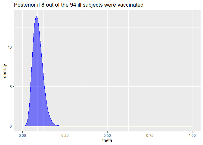
Biontech/Pfizer stated as interim success criterion that the posterior probability of an efficacy below 30% (corresponding to $\theta > 0.4118$) is smaller than 2.5%. We can easily compute this probability with our posterior distribution on $\theta$:

pbeta(0.4118,a,b,lower.tail = FALSE)*100

## [1] 6.399889e-11

Well, as the graph has already suggested, our posterior probability of an efficacy below 30% is almost 0.

We can compute a Bayesian equivalence of the 95%-confidence interval (called credible interval) for $\theta$ by looking at the 2.5% and 97.5% quantiles of our posterior distribution:

theta.ci = qbeta(c(0.025,0.975),a,b)
round(theta.ci*100,1)

## [1]  4.2 15.6

This means given our prior belief and the data, we believe with 95% probability that the probability that an ill subject is vaccinated is between 4.2% and 15.6%.

We can transform these boundaries into a corresponding credible interval for the vaccine effectiveness:

VE.ci = rev((1-2*theta.ci)/(1-theta.ci))
round(VE.ci*100,1)

## [1] 81.6 95.6

This Bayesian credible interval from 81.6% to 95.6% of the vaccine effectiveness is actually quite close to the frequentist confidence interval we have computed in the first post. That’s reassuring.

Of course, the credible interval depends on the assumed prior for $\theta$. A more conservative prior would have been to simply assume a uniform distribution of $\theta$ which is equal to a Beta distribution with shape parameters $a=b=1$. Let us compute the 95% credible interval for this uniform prior:

a0 = b0 = 1
a = a0+8; b = b0+94-8
theta.ci = qbeta(c(0.025,0.975),a,b)
VE.ci = rev((1-2*theta.ci)/(1-theta.ci))
round(VE.ci*100,1)

## [1] 81.1 95.4

It is nice to see that this different prior has only a quite small impact on the credible interval for the vaccine efficacy which is now from 81.1% to 95.4%.

While I typically was sceptical about Bayesian analysis because of the need to specify a prior distribution, I must say that in this example the Bayesian approach looks actually quite intuitive and nice. You should still take my analysis with a grain of salt, however. It is essentially just an educated guess of how Biontech/Pfizer actually performs the analysis. There may well be some statistical complications that I have overlooked.

UPDATE (2020-11-16): One interesting issue I have not yet addressed is how to control for “multiple testing” in our Bayesian setting if one wants to allow that a trial success can already be determined at interim analyses. I have now written a third post that explores this topic.

PS: I also learned about another blog series here about Bayesian methods for analysing the Covid-19 vaccine trials. It illustrates also some advanced R packages like runjags that can be used for more complex Bayesian analyses.