
Here is one more post about Biontech/Pfizer’s vaccine trial. That is because my previous two posts (here and here) have so far ignored one interesting topic: How do Biontech/Pfizer statistically account for interim analyses? Studying this topic gives us also general insights into how adaptive trial designs with multiple success conditions can be properly evaluated.
According to their study plan sufficient vaccine efficacy is established if one can infer that the efficacy is at least 30% with a type I error (wrongly declaring sufficient efficacy) of no more than 2.5%. While the final evaluation shall take place once there are 164 confirmed Covid-19 cases among the 43538 study participants, the plan states that also at intermediate stages of 32, 62, 92, and 120 cases overwhelming efficacy or, if outcomes are bad, futility can be declared.
Here is a screenshot of Table 5 on p. 103 in the study plan that specifies the exact success and futility thresholds for the interim and final efficacy analyses:
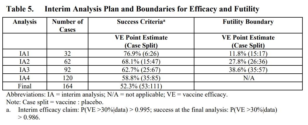
The first interim analysis was planned after 32 confirmed Covid-19 cases. The table states that overwhelming efficacy shall be announced if no more than 6 of these 32 subjects with Covid-19 were vaccinated. Let us draw the posterior distribution of the parameter $\theta$ that measures the probability that a subject with Covid-19 was vaccinated (see the previous post for details):
# Parameters of prior beta distribution
a0 = 0.700102; b0 = 1

# Covid cases in treatment and control group
mv = 6; mc=26

# Compute posterior density of theta
theta.seq = seq(0,1,by=0.01)
density = dbeta(theta.seq,a0+mv,b0+mc)

# Thresholds
VE.min = 0.3
theta.max = (1-VE.min)/(2-VE.min) # 0.41176

ggplot(data.frame(theta=theta.seq, density=density), aes(x=theta, y=density)) +
  geom_area(col="blue", fill="blue", alpha=0.5)+
  geom_vline(xintercept=theta.max) +
  ggtitle("Posterior if from 32 Covid cases 6 were vaccinated")
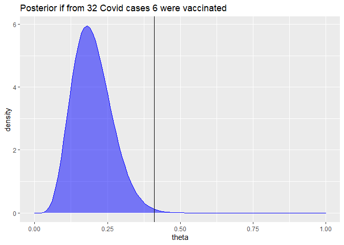
The posterior probability that the efficacy would be above 30% in that case can be simply computed:
prob.VE.above.30  = pbeta(theta.max,a0+mv, b0+mc)
round(prob.VE.above.30*100,3)
## [1] 99.648
This means if the study would have been planned to end after 32 cases with no previous interim evaluation, these thresholds would yield a type I error below 0.352% (i.e. 100% - 99.648%). This is a much stricter bound than the 2.5% type I error bound stated above.
Footnote a) below Table 5, confirms such tighter bounds for the interim analyses:
Interim efficacy claim: P(VE > 30% given data) > 0.995
For the final analysis the footnote also implies an error bound below 2.5%:
success at the final analysis: P(VE > 30% given data) > 0.986.
The crucial point is that the 2.5% bound on the type I error shall hold for the complete analysis that allows to declare sufficient efficacy at 5 different occasions: either at one of the 4 interim analysis or at the final analysis. In a similar fashion as controlling for multiple testing, we have to correct the individual error thresholds of each of the 5 analyses to guarantee an overall 2.5% error bound. The Bayesian framework does not relieve us from such a “multiple testing correction”.
So how does one come up with error bounds for each separate analysis that guarantee a total error bound of 2.5%? For an overview and links to relevant literature you can e.g. look at the article “Do we need to adjust for interim analyses in a Bayesian adaptive trial design?” by Ryan et al. (2020). The article states that in practice the overall error bound of a Bayesian trial design with interim stopping opportunities is usually computed via simulations.
While I want to reiterate that I am no biostatistician, I would like to make an educated guess how such simulations could have looked like.
The following code simulates a trial run until m.max=164 Covid-19 cases are observed, assuming a true vaccine efficacy of only VE.true = 30%:
simulate.trial = function(runid=1, m.max=164, VE.true = 0.3,
    VE.min=VE.true, a0 = 0.700102, b0 = 1, m.analyse = 1:m.max) {
  theta.true = (1-VE.true)/(2-VE.true)
  theta.max = (1-VE.min)/(2-VE.min)

  is.vaccinated = ifelse(runif(m.max) >= theta.true,0,1)

  mv = cumsum(is.vaccinated)[m.analyse]
  mc = m.analyse - mv

  prob.above.VE.min = pbeta(theta.max,shape1 = a0+mv, shape2=b0+mc, lower.tail=TRUE)
  # Returning results as matrix is faster than as data frame
  cbind(runid=runid, m=m.analyse, mv=mv,mc=mc, prob.above.VE.min)
}
set.seed(42)
dat = simulate.trial() %>% as_tibble
dat
## # A tibble: 164 x 5
##    runid     m    mv    mc prob.above.VE.min
##    <dbl> <dbl> <dbl> <dbl>             <dbl>
##  1     1     1     0     1             0.759
##  2     1     2     0     2             0.869
##  3     1     3     1     2             0.618
##  4     1     4     1     3             0.746
##  5     1     5     1     4             0.834
##  6     1     6     1     5             0.893
##  7     1     7     1     6             0.932
##  8     1     8     2     6             0.828
##  9     1     9     2     7             0.881
## 10     1    10     2     8             0.919
## # ... with 154 more rows
Each row of the data frame corresponds to one potential interim analysis after m Covid-19 cases have been observed. The corresponding number of cases from vaccinated subjects mv and from control group subjects mc are random. [Update 2020-11-17: The simulation ignores that if mv and mc increase asymmetrically, the ratio of the remaining healthy subjects in the treatment group vs control group can now slightly differ from the original 1:1 assignment. A more careful simulation should probably account for this effect. But given that there were a large number of subjects (43538) compared to our maximum case count (164, i.e. less than 0.38% of the number of subjects) this simplification hopefully does not matter much.]
The column prob.above.VE.min denotes the posterior probability that the vaccine efficacy is better than VE.min = 30% given the simulated interim data and Biontech/Pfizer’s assumed prior characterized by the arguments a0 and b0. You see how every additional Covid-19 case of a vaccinated subject reduces prob.above.VE.min while every additional Covid-19 case of a control group subject increases it.
Let us plot at these posterior probabilities of a vaccine effectiveness above 30% for all possible interim analyses and the final analysis for our simulated trial:
ggplot(dat, aes(x=m, y=prob.above.VE.min*100)) +
  geom_line() + geom_hline(yintercept = 97.5)
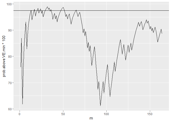
You see how this posterior probability varies substantially. In a few interim analyses the 97.5% threshold is exceeded but not in all. (As you may have guessed from the random seed, this is not a completely arbitrary example. I picked an example where the 97.5% line is actually breached. This happens not in all runs, but it is representative that the posterior probabilities can change a lot between different interim analyses.)
This just illustrates the aforementioned multiple testing problem. Hence, if we allow interim analyses to declare an early success, the critical posterior probability for each separate analysis should be some level above 97.5% to have an overall type I error rate of at most 2.5%.
The simulate.trial function can also simulate the relevant values just for a smaller set of interim analyses, e.g. the five analyses planed by Biontech/Pfizer:
simulate.trial(m.analyse = c(32,64,90,120,164)) %>% as_tibble
## # A tibble: 5 x 5
##   runid     m    mv    mc prob.above.VE.min
##   <dbl> <dbl> <dbl> <dbl>             <dbl>
## 1     1    32    14    18            0.393
## 2     1    64    25    39            0.639
## 3     1    90    40    50            0.270
## 4     1   120    54    66            0.202
## 5     1   164    79    85            0.0364
To assess how error thresholds should be adapted, we repeat the simulation above many times. Ideally, a large number like a million times, but for speed reasons, let us settle with just 100000 simulated trials:
set.seed(1)
dat = do.call(rbind,lapply(1:100000, simulate.trial, m.analyse = c(32,64,90,120,164))) %>%
  as_tibble
We can now compute in which fraction of simulated trials at least one analysis (one of the 4 interim or the final one) yields a posterior probability above 97.5% for a vaccine efficacy above 30%.
agg = dat %>%
  group_by(runid) %>%
  summarize(
    highest.prob = max(prob.above.VE.min),
    final.prob = last(prob.above.VE.min)
  )

# Share of simulation runs in which highest posterior probability
# of VE > 30% across all possible interim analyses is larger than
# 97.5%
mean(agg$highest.prob > 0.975)
## [1] 0.07179
# Corresponding share looking only at the final analysis
mean(agg$final.prob > 0.975)
## [1] 0.02656
While in 2.66% of the simulated trials, the final posterior probability of an efficacy larger than 30% is above 97.5%, we find in 7.18% of the simulated trials at least one interim analysis or the final analysis with that posterior probability above 97.5%.
Assume we want to set in all interim analysis and the final analysis the same threshold for the posterior probability of a vaccine efficacy above 30% so that the total error rate is below 2.5%. We can find the corresponding threshold by computing the empirical 97.5% quantile in our simulated data:
quantile(agg$highest.prob, 0.975)
##     97.5%
## 0.9922456
This means we should accept the efficacy only if in one of the 5 analyses the posterior probability of a vaccine efficacy above 30% is above 99.22%. The more interim analyses we would run, the tougher would be this threshold.
However, there is no reason to set the same threshold for all interim analyses and the final analysis. In their study plan Biontech/Pfizer set a tougher success threshold of 99.5% for the 4 interim analyses, but a lower threshold of 98.6% for the final analysis.
Let us see whether we also come up with the 98.6% threshold for the final analysis if we fix the interim thresholds at 99.5% and want to guarantee a total type I error rate of 2.5%:
agg = dat %>%
  group_by(runid) %>%
  summarize(
    interim.success = max(prob.above.VE.min* (m<164)) > 0.995,
    final.prob = last(prob.above.VE.min)
  )

# Fraction of trials where we have an interim success
share.interim.success = mean(agg$interim.success)
share.interim.success
## [1] 0.01516
# Remaining trials without interim success
agg.remain = filter(agg, !interim.success)

# Maximal share of success in final analysis in remaining trials
# to guarantee 2.5% error rate
max.share.final.success = (0.025-share.interim.success)*
  NROW(agg)/NROW(agg.remain)

quantile(agg.remain$final.prob, 1-max.share.final.success)
## 99.00085%
## 0.9852906
OK, I have not deeply checked that there is no mistake in the computation above, but we indeed get a required threshold for the final trial of 98.53%. If we round it, we must round it up to keep the total error rate bounded by 2.5%, which yields the 98.6% threshold used by Biontech/Pfizer. So possibly, we indeed have replicated the computations that formed their study plan.
Overall, I consider this approach an intriguing mixture between Bayesian statistics and frequentist hypothesis testing. In some sense it feels like the Bayesian posterior distributions are used as frequentist test statistics whose distributions we establish by our simulation.
For the sake of simplicity, I have ignored that the interim analyses also have futility thresholds that can lead to an early stop of the trial. Accounting for this possibly will generate some slight slack in the threshold computed above. But likely the threshold will not change much because I imagine that there are only very few trials that would in some interim analyses be declared futile while (if futility is ignored) in later analyses be declared an overwhelming success.
Giving the degrees in freedom in the number and timing of the interim analyses and in the distribution of critical thresholds across the different analyses, optimal trial analysis design seems like a very interesting applied optimization problem. Of course, solving such an optimization problem would require a lot of estimates like a quantification of gains from earlier conclusions and true subjective beliefs about the efficacy distribution (possibly more optimistic than the conservative priors used for regulatory purposes).
One can also imagine that more flexible adaptive trial designs can be evaluated with similar simulations. E.g. assume that in another vaccine trial one wants to perform the final analysis after say m=100 cases and earlier wants to have exactly one interim analysis, which shall take place at a specific date no matter how many cases mi have accrued at that date. One could then possibly make a valid study plan that just specifies the probability threshold for the interim analysis, like 99.5% while the threshold for the final analysis will be a function of the number of cases mi at the interim analysis and set such that for every possible value of mi a total type error I bound of 2.5% is guaranteed.
As long as one can verify that one has yet looked at the data, one possibly can also adapt the analysis plan in a running study. E.g. Biontech/Pfizer’s press release states:
After discussion with the FDA, the companies recently elected to drop the 32-case interim analysis and conduct the first interim analysis at a minimum of 62 cases. Upon the conclusion of those discussions, the evaluable case count reached 94 and the DMC [independent Data Monitoring Committee] performed its first analysis on all cases.
While we don’t know the chosen thresholds for the modified study plan, it seems obvious from the thresholds of the original design that the vaccine efficacy is established already at the interim analysis with 94 cases. It is also stated in the press release that the clinical trial continues to the final analysis at 164 confirmed cases. However, this shall be done in order to collect further data and characterize the vaccine candidate’s performance against other study endpoints. Submission for Emergency Use Authorization seems still to require a safety milestone to be achieved, but it doesn’t look like proving efficacy is an issue anymore.
As a personal summary, I had not thought that I end up writing three blog posts when I started with the idea to understand a bit better how this famous vaccine trial is evaluated. But with each post I learned new, interesting things about study design and analysis. Hope you also enjoyed reading the posts a bit.
UPDATE (2020-11-16 14:00): I just read the good news from Moderna’s vaccine trial and skimmed over the study plan that Google located. Interestingly, they seem to use a pure frequentist approach in the statistical analysis and the study plan contains terms like Cox proportional hazard regression and O’Brien-Fleming boundaries (for dealing with interim analyses).
Published on 16 Nov 2020 •