
The discussion on how to deal with exploding European electricity prices takes on steam. Recent ideas of the EU and similar proposals by the German government do not directly attempt to reduce electricity wholesale prices. The goal is to collect infra-marginal rents in another way and redistribute the money to energy users by different channels than wholesale price reductions.
The question is whether that approach can in fact be implement without too many inefficiencies and negative unintended consequences. In particular, the hedging problem must be solved.
Thus, perhaps other approaches that try to directly reduce electricity wholesale prices might be coming back on the table. On example are fuel subsidies for gas power plants as implemented in Spain and Portugal.
Besides other problems of such a wholesale price cap, one important risk is that a wholesale price reduction could lead to a substantial increase in electricity demand and gas consumption in the power sector. This could be very detrimental to the crucial necessity to reduce natural gas consumption.
Goal of this post is to get a crude idea of how strongly electricity demand would react if high wholesale prices were reduced.
I have a data set with hourly data on German electricity demand (=load), day-ahead spot market prices, and wind power production (used later for an instrumental variable regression) from 2015 until start of September 2022:
bind_rows(head(dat,3), tail(dat,3))
## # A tibble: 6 x 9
##   time                 load price  wind  hour date        year month wday
##   <dttm>              <dbl> <dbl> <dbl> <int> <date>     <dbl> <ord> <ord>
## 1 2015-01-01 01:00:00  43.5  18.3  9.68     1 2015-01-01  2015 Jan   Thu
## 2 2015-01-01 02:00:00  42.0  16.0  9.83     2 2015-01-01  2015 Jan   Thu
## 3 2015-01-01 03:00:00  40.6  14.6  9.79     3 2015-01-01  2015 Jan   Thu
## 4 2022-09-02 04:00:00  43.6 392.  11.1      4 2022-09-02  2022 Sep   Fri
## 5 2022-09-02 05:00:00  46.0 445.  10.4      5 2022-09-02  2022 Sep   Fri
## 6 2022-09-02 06:00:00  51.3 532.  10.0      6 2022-09-02  2022 Sep   Fri
Monthly averages
Let us take a look at the development of average monthly prices and load over time:
modat = dat %>%
  group_by(year, month) %>%
  summarize(
    date = first(date),
    price = weighted.mean(price,load),
    load = mean(load)
  )

ggplot(modat, aes(x=date)) +
  geom_line(aes(y=price), col="red", size=1) +
  # Scale load by factor 5 to better compare both lines
  geom_line(aes(y=load*5), col="blue", size=1) +
  xlab("Date") +
  annotate("text", x=as_date("2016-01-01"), y=350, label= "Load", col="blue") +
  annotate("text", x=as_date("2020-01-01"), y=100, label= "Spot Market Price", col="red") +
  scale_y_continuous(breaks = seq(0, 500, by=50),
  sec.axis = sec_axis(~./5, name="GW"))+
  ylab("EUR / MWh") +
  #theme(axis.text.y=element_blank(), axis.ticks.y=element_blank()) +
  ggtitle("Average Hourly Spot Market Prices and Load")

Prices strongly increased in 2021 and 2022. Before summer 2022, I cannot see any reduction in load. Also any reduction in summer 2022 that goes beyond the seasonal fluctuations seems quite small compared to total electricity demand.
Let’s look at data for August (our last month in the data set) in the different years:
modat %>%
  filter(month=="Aug")
## # A tibble: 8 x 5
## # Groups:   year [8]
##    year month date       price  load
##   <dbl> <ord> <date>     <dbl> <dbl>
## 1  2015 Aug   2015-08-01  32.6  53.8
## 2  2016 Aug   2016-08-01  27.9  53.9
## 3  2017 Aug   2017-08-01  31.8  53.9
## 4  2018 Aug   2018-08-01  57.2  55.4
## 5  2019 Aug   2019-08-01  37.7  53.2
## 6  2020 Aug   2020-08-01  35.7  51.3
## 7  2021 Aug   2021-08-01  84.5  53.4
## 8  2022 Aug   2022-08-01 470.   52.9
Compared to the Pre-Covid mean from 2015-2019 of 54 GW, the hourly load in Aug. 2022 is 52.9 GW, i.e. only 2 percent lower. In contrast, average prices in August increased roughly 13-fold from 36.5 Euro/MWh (2015-2019) to 465 Euro / MWh in 2022.
At least this data does not show that average German electricity demand is fairly elastic with respect to average spot market prices. Regulations that reduce spot market prices may thus perhaps only yield an acceptable small increase in electricity demand.
Yet, the reason that we observe such a small demand reaction could be that many electricity consumers have longer term fixed-price contracts. (That seems definitely the case for most German households). This means the high prices may just not have reached many consumers, yet. In longer time series, we could see a stronger demand reaction.
Hourly data
Looking at monthly average prices does not tell us how flexibly demand reacts to short term price fluctuations. For example, consider a day with a lot of solar production and low prices in the afternoon but high prices and a lot of gas production in the early evening. We would love that demand is sufficiently flexible and substantially shifts away from such high price hours, in which gas power plants run, to low price hours with a lot of renewable production.
It seems not easy to estimate the existing extend of demand flexibility just by looking at market data on prices and output. In this post, I want to “just” look at estimating how hourly electricity demand is reduced by high spot market prices without assessing how much of demand reduction is shifted to hours with lower prices that day. As we will see, also the answer to this simpler question can already differ substantially depending on the exact approach, including functional form assumptions.
Some background on the estimation approach
(You can skip this section if you know IV regression)
Let us first look at the relationship between hourly demand and spot market prices in the pre-crisis year 2019:
d = dat %>%  filter(year == 2019)
ggplot(d, aes(x=price, y=load, fill=wind,color=wind)) +
  geom_point() + geom_smooth(se=FALSE, color="red")
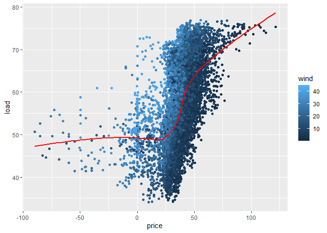
We see on average a positive relationship between load and prices. Does that mean higher prices lead to higher demand? Of course not. The positive relationship is due to a reverse causal effect: higher demand leads to higher prices. We have a so called endogeneity problem.
Adding control variables for factors related to demand fluctuations, like certain time fixed effects for month, weekday and hour of the day can reduce the endogeneity problem. I will do so, but it does not suffice to solve the endogeneity problem. In addition, I will use the instrumental variable method. Let me try to explain the key idea somewhat informally.
For instrumental variable estimation, we need a variable (the instrument) that influences prices but after controlling for the time fixed effects is uncorrelated with other factors that influence demand. I choose electricity production from wind power production as instrument.
In the scatter-plot above a lighter color corresponds to an hour with more wind power production. We see how hours with higher wind production tend to have lower prices. That is good.
As a valid instrument, wind should not be correlated with demand fluctuations, except for those caused by different prices or those explained by the time fixed effects that we control for. In the scatter-plot, we see a small positive correlation with wind production and load. But that correlation may well just reflect the actual effect of lower prices on demand or seasonal fluctuations that we control for.
Thus in my estimations below, I will use wind power production as instrument for the electricity production.
While there are several R packages that allow to directly perform instrumental variable estimation, it is helpful to understand how one could implement the procedure with the so called two-stage least squares (2SLS) method.
-
In the first stage, regress the endogenous variable
priceon the instrumentwindand the other control variables (here time fixed-effects). Then compute the predicted valueprice.hatfrom this regression. -
In the second stage, estimate the original demand specification via OLS with one important difference: replace the endogenous explanatory variable
pricewith the fitted valuesprice.hatfrom the first stage regression.
First specification: a linear demand function
Let us estimate a simple linear demand function controlling for year-month, weekday and hour of day fixed effects, using wind power production as instrument for the endogenous price. The code below estimates the two stages of the 2SLS approach using the fixest package. (The fixest package allows considerably speed up in regressions with lot of fixed effects).
# Generate variable for date and time fixed effects
dat$year_month = paste0(dat$year,"_", dat$month)
dat$hour_of_day = as.character(dat$hour)

# 1st stage regression with fixest
library(fixest)
reg1 = feols(price ~ wind | year_month+wday+hour_of_day, data=dat)

# Save the predicted price in price.hat
dat$price.hat = fitted(reg1)

# 2nd stage regression
reg2 = feols(load ~ price.hat | year_month+wday+hour_of_day, data=dat)
coef(reg2)
##   price.hat
## -0.04237639
We estimate a coefficient of -0.042. This means an increase of spot market prices by 100 Euro is expected to reduce load by 4.2 GW. On the one hand, this may look like a very small effect, given that in the used data set from 2015 to 2022 average spot prices were 62 Euro / MWh and average load 57 GW.
On the other hand, consider a situation were without the price cap spot market prices were 1200 Euro / MWh. Then taking these estimates at face value, introducing a price cap of 600 Euro / MWh would mean that the price cap increases demand by a whopping 25.2 GW in that hour.
For me the model’s predictions do not seem very plausible at such high electricity prices. That gut feeling is supported by the almost non-visible demand reaction in our monthly averaged data further above. I think there are two related problems with the specification above if our goal is to understand how demand reacts at high very price levels:
-
Many data points are at low price levels. E.g. in 79% of observations the price is below 60 Euro / MWh. This means changes in demand at low price levels determine to a large extend our regression results. But what information can we learn from those data points about how a price cap that would reduce a market price of say 1200 Euro / MWh to 600 Euro / MWh affects demand?
-
The functional form assumption of a linear demand function probably yields a quite poor extrapolation when looking at effects at high price levels.
A specification with selected sample and different functional form
In the next specification, I want to address both points.
Sample choice
First, I would like to use a selected sample that concentrates on hours with higher electricity prices.
We might think of using only the observations were the price was above some threshold like 300 Euro / MWh. Yet, selecting a sample based on the value of an endogenous explanatory variable is probably a bad idea and might generate biases even in an instrumental variable regression. (I am not 100% sure that it is indeed a problem, but I am less sure that it is no problem.)
Hopefully, it is not problematic though, to select our sample based on the value of our predicted price price.hat from the first stage regression, as it is a linear combination of exogenous variables. (If any statistician / econometrician reads this and can confirm or reject my guesses, I am happy for a short note via email.)
Unfortunately, we have no observations in our data set with a predicted price above 600 Euro / MWh. So let us use for our sample the 1400 observations with a predicted price above 300 Euro / MWh.
sample300 = filter(dat, price.hat >= 300)
range(sample300$time)
## [1] "2022-07-01 00:00:00 CEST" "2022-09-02 06:00:00 CEST"
It actually turns out that this sample corresponds to all the observations from July 2022 onward, where we have large year_month fixed effects in the first stage regression and thus high predicted prices. Actually, just taking these most recent data points in our sample might be not a bad selection. So let’s continue with this sample.
Functional form (logs!)
If one beliefs that across price levels a same percentage change of prices will roughly have the same percentage effect on demand, one would typically use a specification in logs, i.e. use log(load) as dependent variable and log(price) as explanatory variable.
One problem is that log’s are only specified for positive numbers. Let’s look at the range of prices:
range(dat$price)
## [1] -130.09 871.00
range(sample300$price)
## [1] 13.29 871.00
In the complete data set, we could not directly apply the log transformation due to negative electricity prices in some periods. Yet, fortunately, all electricity prices are positive in our sample.
I now directly run the IV regression using the function iv_robust from the estimatr package. (The feols function from fixest also allows direct IV regression and would be faster. But later I want to use the predict function and did not manage to make it work correctly with feols.)
library(estimatr)
iv300 = iv_robust(log(load) ~ log(price)+ year_month+wday+hour_of_day |
  wind+ year_month+wday+hour_of_day, data=sample300, se_type="HC1")

broom::tidy(iv300, conf.int=TRUE)[2,]
##         term   estimate  std.error statistic      p.value   conf.low
## 2 log(price) -0.1026856 0.01564861  -6.56196 7.516985e-11 -0.1333835
##     conf.high   df   outcome
## 2 -0.07198768 1367 log(load)
We get an estimate of -0.10 in the log-log specification, which can be interpreted as a short-run demand elasticity of electricity. This means we estimate that a 1% increase of an hourly spot market price yields roughly a 0.1% reduction in electricity demand in that hour. Looks like a plausible number.
But just because a number looks plausible does not imply that we have a robust results.
For example, how would our specification change if we use as sample all 3784 observations with a predicted price above 200 Euro / MWh?
sample200 = filter(dat, price.hat >= 200)
range(sample200$price)
## [1] -19.04 871.00
Hmm, now we also have negative prices in our sample. If we simply use log(price) in our regression specification, R would just drop all observations with negative prices. But then we would base our selection on the endogenous variable, which we probably should not do. Hence, I do something different in the following code:
iv200 = iv_robust(log(load) ~ log(price+20)+ year_month+wday+hour_of_day |
  wind+ year_month+wday+hour_of_day, data=sample200, se_type="HC1")
broom::tidy(iv200, conf.int=TRUE)[2,]
##              term    estimate   std.error statistic    p.value   conf.low
## 2 log(price + 20) -0.01347163 0.006183256 -2.178727 0.02941412 -0.0255945
##      conf.high   df   outcome
## 2 -0.001348749 3744 log(load)
We now get an estimated coefficient of -0.013. The interpretation is as follows: If the sum of price and 20 Euro / MWh changes by 1%, we estimate that demand goes down by approximately just 0.013%. When looking at high prices just adding 20 Euro / MWh has no big effect on how much a 1% change is. So here we estimate an effect that is roughly one order of magnitude smaller than in our previous specification.
Comparing all 3 specification for a price change from 1200 Euro / MWh to 600 Euro / MWh
Finally, I want to use some R code to more precisely compare the predictions of the three specifications we looked at. First, I generate two observations, for which I want to predict demand:
pdat = dat[c(67162,67162),]
pdat$price = c(600,1200)
select(pdat, time, price, load, wind)
## # A tibble: 2 x 4
##   time                price  load  wind
##   <dttm>              <dbl> <dbl> <dbl>
## 1 2022-08-31 18:00:00   600  58.7  9.00
## 2 2022-08-31 18:00:00  1200  58.7  9.00
I basically, created two rows from one sample observation: in the first row I consider a price of 600 Euro / MWh and in the second row a price of 1200 Euro / MWh.
As next step, I re-estimate the linear model with iv_robust so that I can use the predict function afterward.
# Re-estimate linear specification in order to use predict
iv.lin = iv_robust(load ~ price+ year_month+wday+hour_of_day |
  wind+ year_month+wday+hour_of_day, data=dat)
Now I predict, for each regression specification the load given the two prices, and compute by how much predicted load increases when reducing the fictitious price of 1200 Euro / MWh to 600 Euro / MWh.
comp.load.reduction = function(reg, label, log = FALSE) {
  if (log) {
    pred.load = exp(predict(reg, pdat))
  } else {
    pred.load = predict(reg, pdat)
  }
  tibble(label, load.reduction=paste0(round(100*(pred.load[1]-pred.load[2]) / pred.load[1],1),"%"))
}

bind_rows(
  comp.load.reduction(iv.lin, "linear"),
  comp.load.reduction(iv300, "log, p.hat >= 300", log=TRUE),
  comp.load.reduction(iv200, "log, p.hat >= 200", log=TRUE)
)
## # A tibble: 3 x 2
##   label             load.reduction
##   <chr>             <chr>
## 1 linear            44.4%
## 2 log, p.hat >= 300 6.9%
## 3 log, p.hat >= 200 0.9%
We have largely different estimates ranging from a load reduction of 44.4% in our linear specification, to 0.9% load reduction in our last specification. Sure the 6.9% in the center may look like the most plausible result. But honestly the wide range of estimates suggests that it is extremely difficult to predict with our data from a time of relatively low prices how hourly demand reacts to prices at much higher price levels.
We also don’t know yet, to which degree demand would only shift within a day and to which hours. Yet, given the uncertainties across the specification in the estimation above, I will currently refrain from further exploration of this question.
Published on 07 Sep 2022 •